Part 6:
STK Pro, STK Premium (Air), STK Premium (Space), or STK Enterprise
You can obtain the necessary licenses for this training by contacting AGI Support at support@agi.com or 1-800-924-7244.
This lesson is an introduction to STK's Pro capability. Pictures, graphs, and data snippets are used as examples only. The results of the tutorial may vary depending on the user settings and data enabled (online operations, terrain server, dynamic Earth data, etc.). It is acceptable to have different results. Throughout the tutorial, there are hyperlinks that take you to the appropriate STK Help area which further expand your knowledge on the subject.
Credits: ISERV, NASA
Capabilities Covered
This lesson covers the following STK Capabilities:
- STK Pro
Problem Statement
Engineers and operators require a quick way to determine if local terrain is affecting visibility between ground sites and satellites for a variety of purposes such as communications, imaging, and general situational awareness. In this tutorial, there is a GPS monitoring station in the vicinity of Mount St. Helens. A USGS Digital Elevation Model (DEM) file contains terrain data for the area requiring analysis. Raw satellite imagery is available of Mount St. Helens which will provide situational awareness of the analytical area when converted as an inlay. A further need exists to create color elevation imagery of the area to be used in a briefing and in documentation.
Solution
Using STK, load a DEM file to analyze the impact of local terrain on accesses between a ground station and GPS satellites. Create a color elevation image, and convert a raw satellite image that can be used as an inlay for visualization and situational awareness. Change the DEM file into a STK Terrain File (pdtt) which can be used to visualize terrain in the 3D Graphics window.
Upon completion of this tutorial, you will be able to:
- Use terrain data for analysis and visualization
- Build a Constellation object
- Build a Chain object
Video Guidance
Watch the following video. Then follow the steps below, which incorporate the systems and missions you work on (sample inputs provided).Create a New Scenario
Create a new scenario with a run time of twenty four (24) hours.
- Launch STK (
 ).
). - Click the Create a Scenario (
 ) button.
 - Enter the following in the STK: New Scenario Wizard:
- When you finish, click OK.
- When the scenario loads, click Save (
 ). A folder with the same name as your scenario is created for you.
 - In the Save As window, verify the scenario name and location and click Save.
| Option | Value |
|---|---|
| Name: | STK_Pro |
| Start: | Default |
| Stop: | Default |
Save Often!
U.S. Geological Survey Data
The DEM file used in this tutorial is located in the install directory. Take a moment to download the file. DO NOT unzip the folder. Follow the instructions in the tutorial to use the file.
- Create a folder on your Desktop called Terrain.
- Browse to the location of the DEM file using the following:
- STK 11: C:\Program Files\AGI\STK 11\CodeSamples\CodeSamples.zip\SharedResources\Scenarios\Events
- STK 12: C:\Program Files\AGI\STK 12\CodeSamples\CodeSamples.zip\SharedResources\Scenarios\Events
- Locate and copy the file named hoquiam-e.dem.
- Paste the hoquiam-e.dem file into the Terrain folder you created on your desktop.
Analytical Terrain
The Pro capability adds realism to system models. Building on the fundamental capabilities of STK, Pro introduces more sophisticated modeling through advanced access constraints, flexible sensor shapes, complex visibility links, more object tracks and digital terrain data.
Load the locally available DEM terrain data file to be used for analysis and visualization into the scenario.
- Open STK_Pro's () properties.
- Select the Basic - Terrain page.
- Disable Use terrain server for analysis.
- In the Custom Analysis Terrain Sources field, on the right, click Add.
- When the Open window appears, change Files of type: to USGS DEM (DEM).
- Browse to the Terrain folder containing the hoquiam-e.dem file.
- Select hoquiam-e.dem and click Open.
- Click OK in the properties window to load the hoquiam-e.dem file as analytical terrain.
You're using a local terrain file for both analysis and visualization. By turning off streaming terrain, you are simulating what you'd see in a setting that doesn't have an Internet connection.
Terrain Regions Display
Display an outline around the imported terrain region on the 2D Graphics window. The following turns off Bing maps and switches to the default Basic.bmp. If you don't have an Internet connection, this is the default map.
- Bring the 2D Graphics window to the front.
- Open the 2D Graphics window's properties (
 ).
). - On the Imagery page, enable Image File: and ensure Basic.bmp is selected (default).
- Select the Details page.
- In the Map Details field, click on and highlight the following (leave RWDB2_Coastlines highlighted):
- RWDB2_International_Borders
- RWDB2_Provincial_Borders
- In the Terrain Regions Display field, enable Show Extents.
- Click OK.
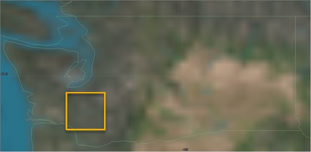
- Bring the 2D Graphics window to the front and zoom in to the state of Washington.
- Zoom in to the terrain extents.
The following will outline international borders and all the states of the United States and provinces of Canada.
Finally, create a yellow outline of the hoquiam-e.dem file's location.
The yellow box in the southwest corner of the state is the location of the hoquiam-e.dem file. Analysis inside the box can be done using local terrain. Analysis outside the box will take place on the WGS84.
Show Extents
Color Elevation Imagery
The Create Color Elevation Imagery utility allows you to create images from terrain data that show elevation data colored by height (for example, blue for sea level, green for land, and white for mountain tops). This is useful if you need to visualize terrain but lack imagery or if you want to put the emphasis on height rather than the content of the image.
- On the 2D Graphics window, zoom in to the terrain region display and move it to the right of your map.
- Open the Utilities menu and select Create Color Elevation Imagery.
- When the Create Color Elevation Imagery utility opens, move it next to the terrain region display.
- Enter the following extents which match the hoquiam-e.dem extents:
- Click the Get Min/Max Altitude button.
- Set the following Min Altitude: values:
- Change Output File / Format to JPEG 2000 Image (jp2).
- Click the Directory: ellipses button and browse to the location of your scenario (e.g. C:\Users\username\Documents\STK 12\STK_Pro).
- Change Filename: to "StHelensColor".
- Click Convert.
- Close the Create Color Elevation Imagery utility.
| Option | Value |
|---|---|
| North Lat | 47 deg |
| West Lon | -123 deg |
| East Lon | -122 deg |
| South Lat | 46 deg |
Displays the minimum and maximum altitude values of the region selected in the 2D Graphics window. This range can help if you use explicit colors. Set HSV for the rendering of elevation data during the conversion process. The resulting image is colored so that elevations are drawn with a linearly interpolated color between the minimum altitude and the maximum altitude, depending on the elevation. Change the minimum altitude values. The default values create a dark blue color. You are landlocked so use a corresponding HSV code that removes the blue.
| Option | Value |
|---|---|
| Hue | 0.25 |
| Saturation | 0.75 |
| Value | 0.20 |
2D Graphics Imagery
2D Graphics Imagery is used to display a background image and inlay images in 2D Graphics windows.
- Bring the 2D Graphics window to the front.
- Open the 2D Graphics window properties ().
- On the Imagery page, locate the Inlay Images field and click the Add button.
- Select the file StHelensColor.jp2.
- Click Open.
- Click OK.
Lower elevations are darker in color and higher elevations are lighter in color. Mount St. Helens sticks out as the highest point in the image.
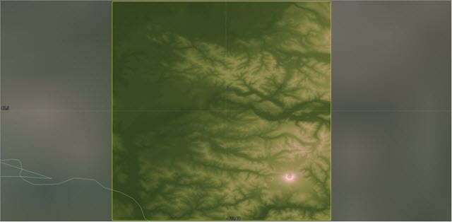
Color Elevation Image
Imagery and Terrain Converter
Use the Imagery and Terrain converter to convert a single image, with or without terrain data, into a format that can be displayed in a 3D Graphics window. The image is converted to a pdttx or jp2 file (image inlay) and the terrain data is converted to a pdtt file (terrain inlay).
Imagery
Convert an ISS SERVIR Environmental Research and Visualization System (ISERV) LEVEL-R (RAW) imagery .jpg into JPEG 2000 Image (jp2) inlay.
- Open the Utilities menu and select Imagery and Terrain Converter.
- In the Input Data field, click the Image Filename: ellipses button.
- Browse to the location of the ISERV imagery. (Typically, <STK install folder>\Data\Resources\stktraining\imagery\)
- Open the folder named ISERV_Imagery.
- Select the file named IPR201407092040194622N12217W.JPG and click Open. The extents are automatically read from the metadata contained in the supporting files.
- In the Output Data field, make the following Image File changes:
- Click Convert.
| Option | Value |
|---|---|
| Format: | JPEG 2000 Image (jp2) |
| Directory: | Location of the scenario (e.g. C:\Users\username\Documents\STK 12\STK_Pro |
| Filename: | ISERV_StHelens |
Terrain
Convert the hoquiam-e.dem file into a STK Terrain File (pdtt).
- In the Imagery and Terrain Converter, select the Terrain Region page.
- In the Input Data field, open the Terrain Source: pull down menu.
- Select the path to the hoquiam-e.dem file.
- In the Output Data field, make the following changes:
- Click Convert.
- Close the Imagery and Terrain Converter.
| Option | Value |
|---|---|
| Directory: | Location of the scenario (e.g. C:\Users\username\Documents\STK 12\STK_Pro |
| Filename: | StHelensTerrain |
Globe Manager
Globe Manager allows you to customize scenario globes with imagery and terrain data as well as manage that data once it has been applied. The Hierarchy window is used to add central bodies, image and terrain items to a scenario.
- Bring the 3D Graphics window to the front.
- In the 3D Graphics window toolbar, click the Globe Manager (
 ) icon. Globe Manager is docked below the Object Browser.
 - In the Hierarchy toolbar, click the Add Terrain/Imagery (
 ) icon.
 - When the pop up window appears, select Add Terrain/Imagery.
- When the Globe Manager: Open Terrain and Imagery Data window opens, ensure Local Files is selected.
- Open the Path: pull down menu and select the path to your scenario (e.g. C:\Users\username\Documents\STK 12\STK_Pro).
- Select both the Image (ISERV_StHelens.jp2) and Terrain files (StHelensTerrain.pdtt).
- Click Add.
- When the Use Terrain for Analysis window appears, select No. You're already using the hoquiam-e.dem file for analysis.
- In Globe Manager, right-click on ISERV_StHelens.jp2 and select Zoom To.
- Use your mouse to view the image and surrounding terrain.
- When finished, ensure the ISERV_StHelens.jp2 and StHelensTerrain.pdtt are turned on.
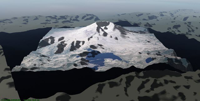
ISERV Imagery on top of PDTT file.
You can see the satellite image ISERV_StHelens.jp2 which is placed on top of the StHelensTerrain.pdtt. Terrain outside of the image is still visible. If desired, you can return to Globe Manager and turn Aerial.ve back on to use Bing Maps. You can also, toggle ISERV_StHelens.jp2 or StHelensTerrain.pdtt on and off to see the visual difference. The ISERV_StHelens.jp2 image can also be used as an inlay in the 2D Graphics window.
Insert the GPS Tracking Device
Insert a Place (![]() ) object which will simulate the GPS satellite tracking device.
) object which will simulate the GPS satellite tracking device.
- Using the Insert STK Objects Tool (
 ) insert a Place (
 ) object using the Insert Default () method.
 - In the Object Browser, name the Place () object "TrackingDevice".
- Open TrackingDevice's () properties ().
- On the Basic - Position page, set the following:
- The tracking device is on a stand and is five (5) feet above the terrain. Set Height Above Ground: to 5 ft.
- Click Apply.
| Option | Value |
|---|---|
| Latitude: | 46.204 deg |
| Longitude: | -122.188 deg |
Define an Azimuth-Elevation Mask
The AzElMask properties enable you to define an azimuth-elevation mask for the GPS tracking device.
- Select the Basic - AzElMask page and set the following:
- Click Apply.
| Option | Value |
|---|---|
| Use: | Terrain Data |
| Use Mask for Access Constraint | Enable |
Selecting Terrain Data automatically creates and stores an azimuth-elevation (Az-El) mask file, which is an ASCII text file that is formatted for compatibility with STK and ends in an .aem extension, into your scenario folder. Turning on Use Mask for Access Constraint enables the Az-El Mask constraint located on the Constraints - Basic page. Using the Az - El Mask constraint constrains access to the object by azimuth-elevation masking which is a 360 degree field of view around the object being constrained.
Display the Azimuth-Elevation Mask
For situational awareness, you can display the Azimuth-Elevation Mask in both the 2D Graphics and 3D Graphics windows.
- Select the 2D Graphics - AzElMask page and set the following At Range properties:
- Click OK.
- Bring the 3D Graphics window to the front.
- Open the 3D Graphics window's properties ().
- On the Details page, turn on Label Declutter - Enable.
- Click OK.
- Right-click on TrackingDevice () in the Object Browser and select Zoom To.
- Using your mouse, zoom out until you can see the visual representation of the Azimuth-Elevation Mask.
| Option | Value |
|---|---|
| Show | Enabled |
| Number of Steps: | 10 |
| Minimum Range: | 0 |
| Maximum Range: | 50 km |
Label Declutter is used to separate the labels on objects that are in close proximity for better identification in small areas. It also keeps object labels from being hidden by terrain.
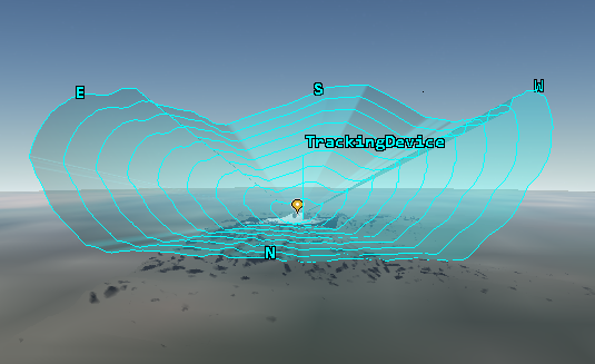
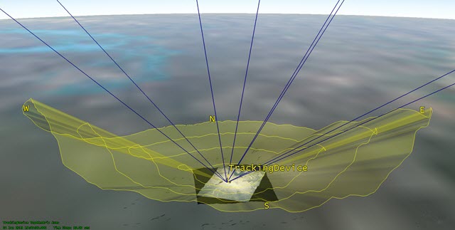
Az El Mask
Each ring represents a ten (5) kilometer range out to fifty (50) kilometers. Around the edge of the view, you can see indications of North (N), South (S), East (E), and West (W). The view indicates that the view to the east, west, and south are poor. Visibility to the north is good.
Constellation Objects
Use the Insert STK Objects tool to load the GPS Constellation using orbital elements from GPS almanac files. The Almanac files can be stored in local directories or pulled from AGI Servers (internet connection required). STK creates a constellation that includes all of the satellites in the almanac. Keep in mind, you can build Constellation (![]() ) objects yourself by loading an empty Constellation (
) objects yourself by loading an empty Constellation (![]() ) object and assigning objects required for your analysis.
) object and assigning objects required for your analysis.
- Using the Insert STK Objects Tool () insert a Satellite (
 ) object using the Load GPS Constellation (
 ) method.
 - Open GPSConstellation's (
 ) properties ().
 - Select the Constraints - Basic page.
- In the Logical Restriction field, set 'From' access position: to At Least N and the value to 4.
- Click OK.
Once loaded, you will see each individual Satellite (![]() ) object and a Constellation (
) object and a Constellation (![]() ) object containing all of the satellites.
) object containing all of the satellites.
On the Basic - Definition page, you can see each GPS satellite has been moved to the Assigned Objects list. If required, you could remove any satellites from the list that are down or are not required for analysis.
For the purposes of this problem, you require access to at least four (4) GPS satellites at any given time. It doesn't matter which four. Also, take into account that when performing an access, the access will be analyzed from the satellite to the GPS tracing device.
Chain Objects
A Chain object is a list of objects (either individual or grouped into constellations) in order of access.
- Using the Insert STK Objects Tool () insert a Chain (
 ) object using the Define Properties () method.
 - On the Basic - Definition page, move (
 ) GPSConstellation from the Available Objects list to the Assigned Objects list.
 - Next, move () TrackingDevice from the Available Objects list to the Assigned Objects list.
- Click OK.
- In the Object Browser, rename the Chain () object "GPStoDevice".
- Bring the 3D Graphics window to the front.
- Zoom To TrackingDevice.
- Using your mouse, zoom out until you can see accesses from the ground site to the GPS satellites.
- Click the Start (
 ) icon in the Animation Toolbar and animate the scenario. Notice how the accesses don't appear until they're above the Az El Mask. Conversely, they disappear when they reach the Az El Mask. Terrain is being taken into account for the accesses.
 - When finished, Reset (
 ) the animation.
Chain Accesses
Complete Chain Access
The Complete Chain Access report shows times during which access among all objects in a chain is possible through one or more strands. Analyze a complete chain access.
- In the Object Browser, right-click on GPStoDevice () and select the Report & Graph Manager.
- When the Report & Graph Manager opens, go to the top of the Styles list and turn off Show Reports.
- In the Styles list, select the Complete Chain Access graph and click the Generate button.
- Close the Graph.
The Complete Chain Access graph might seem boring, but it's telling you exactly what you need to know. If there is a solid line across the report, that means you always have access to at least four (4) or more GPS satellites during the entire analytical period. If there is a break in the line, that's a period when three (3) or less GPS satellites are being accessed.
Individual Strand Access
A Individual Strand Access report represents one possible access pathway through the chain. For a chain that consists of a series of individual objects, only a single strand is possible. If a chain contains one or more constellations, multiple strands are possible, but constellation constraints (ANY OF, ALL OF, AT LEAST N, EXACTLY N) can affect the possible number of strands.
- Return to the Report & Graph Manager.
- In the Styles list, select the Individual Strand Access graph and click the Generate button.
- This graph shows you when the ground site can see individual GPS satellites when that satellite is paired up with at least three more satellites.
- Keep the graph open.
- Open TrackingDevice's () properties ().
- Select the Constraints - Basic page.
- Turn off Az-El Mask.
- Click Apply.
- Return to the Individual Strand Access graph and refresh (
 ) the graph.
 - Return to TrackingDevice's () properties ().
- Turn Az-El Mask back on.
- Click OK.
- Return to the Individual Strand Access graph and refresh () the graph.
Notice how the individual strands grow larger, because the surrounding terrain is no longer being used in the analysis.
The individual strands shrink because analytical terrain is being used in the analysis.
Save Your Work
- When finished, Reset () the scenario and close any reports or tools that are still open.
- Save () your work.
On Your Own
Should you use AzEl Mask or Terrain Mask? Make sure to read the PROs and CONs between the two. When using a Facility, Place or Target object in an access computation, obscuration of the line of sight by terrain can be accounted for in one of two ways: selection of the Terrain Mask constraint or selection of the AzEl Mask constraint. While both constraints serve to model the same physical obstruction, there are important differences between the constraints which should be considered when selecting between the two. Try using Terrain Mask instead of Az-El Mask as a constraint and compare the differences in your reports or graphs and the difference in calculation time.
Also, you could enable Terrain Server and enable either Line-Of-Sight Terrain Mask or Azimuth/Elevation Mask. Place a ground site anywhere on the globe and access a satellite of your choice. Make sure to tell the ground site to use terrain. Try accessing a Ground Vehicle (![]() ) object or an Aircraft (
) object or an Aircraft (![]() ) object as it moves through terrain. Have fun!
) object as it moves through terrain. Have fun!